Part 4: Model Selection
This post is the fourth and last in a series of posts based on chapters in my PhD thesis. The first one is here, the second one is here, and the third one is here.
This last post in my thesis series covers the topic of model selection. As shown in the last two posts, the biexponential and kurtosis models can be affected by ill-conditioning such that the parameter estimates returned by fitting some data can be highly uncertain and may not converge to the true value upon repeated sampling. However, as we saw in these posts, ill-conditioning happened in simulated data when the true signal was close to a monoexponential decay signal. I noted in my previous posts that the biexponential and kurtosis models are extrapolations of the monoexponential signal, with extra parameters/terms included to assess additional phenomena in the signal. When these phenomena aren’t present in the signal, these more complex models have problems with estimation. Extra measures, such as the bootstrap, were needed to determine when these problems were present. Application of these more complex models to signals that are better described by a simpler model illustrate a problem called model misspecification. This seems obvious in retrospect - why bother using these more complex models when the simple, monoexponential model is the obvious model and is already a clinical standard? Unfortunately when measuring human tissue, we usually don’t know what the underlying signal is and, therefore, which model should be specified for use. Thus, studies are often done using model selection techniques to determine which model may be more appropriate for a given tissue. The most common model selection techniques seen in the diffusion MRI literature are statistical tests, cross-validation, or information criteria.
Cross-Validation
Cross-validation is a model selection technique that is seen in several studies in the diffusion MRI literature, and is more widely found in the machine learning literature and community. For machine learning, cross-validation consists of dividing up your entire set of data into a “training” set and a “test” set. Models are optimized by fitting the data in the training set, taking that set of parameters and then assessing that performance on the remaining data in the test set. In many machine learning applications, the dataset can consist of thousands or even millions of data points, so this cross-validation can be performed multiple times with different training/test set combinations, and the model parameters optimized. This can also be used to determine if one model fits or describes the data better than another. Unfortunately, in diffusion MRI data, we are lucky if the data set (b-value measurements) number in the “tens”, so we often use a method called leave-one-out cross-validation (LOOCV). In LOOCV, we leave the first data point out of our set, fit the data with a specific model, and calculate the Mean Squared Error (MSE) associated with that fit. The MSE is essentially a measure of how well the model fits the data. We then rotate the data point that is left out to the second one, fit and add that MSE value to the total. After cycling through all data points left out, we take the total MSE for that model and compare it to the total MSE values for all models being fit to that data. The lowest total MSE signifies the best-fitting model, so we can conclude that for this particular data set, that model will give the best performance. The downside of LOOCV testing is that it requires additional computing time, so testing each of the ten data points requires ten fits in addition to the original regression fit of all ten data points, leading to an elevenfold increase in computing time.
Statistical Test
In the context of model selection between two models, a statistical test is often used as a hypothesis test, where the null hypothesis is that one model does not provide a superior fit to the other. An example of this is the F-test, where we can compare two models with the simpler model often nested within the more complex model. For our models, let’s say that we want to compare the biexponential and monoexponential model on a given data acquisition from a single voxel. If we perform a regression fit on the data using each model and take the Residual Sum of Squares (RSS) value from each fit, we can compare the fits using the following formula
F = [(RSSmono − RSSbiexp)/RSSbiexp]/[(kbiexp − kmono)/(n − kbiexp)]
where k is the number of parameters in each model and n the number of data points. The value of F is then compared to a standardized value from an F distribution. I used the function finv in MATLAB with the numerator degrees of freedom set to (kbiexp − kmono) and the denominator degrees of freedom set to (n − kbiexp). Algorithmic tests like MATLAB’s finv test will return a p-value, which can then be compared to a pre-designated significance level (α), often set to 0.05. Feel to review my discussion of p-values in my introductory post if so desired. If the p-value is less than the pre-set significance level, then the hypothesis that there is no difference between the two model is rejected, often interpreted as the biexponential model being a better fit than the monoexponential model. The downside of the statistical hypothesis test is that only two models can be compared at the same time. Furthermore, the biexponential and kurtosis model aren’t nested within each other, so they can’t be compared to each other using this method.
Information Criteria
There are several different information criteria found in the statistical literature, but the one that is most often seen, at least in the diffusion MRI literature is the Akaike Information Criterion (AIC). The AIC is another method that is used compare models, and the “information” label comes from the fact that the AIC measures the information loss when a model is used to fit a set of data. The basic form of the AIC is the equation
AIC = -2 log(L) + 2k
where L is the likelihood function and k the number of parameters in a given model used in that likelihood function. Since I used regression fitting for nearly my entire thesis, I used a form of the AIC equation which uses the RSS values returned by a regression fit
AIC = n log (RSS/n) + 2k
where n is the number of data points being fit in the regression. The two terms of the AIC equation represent the dichotomy of model fitting known as the bias-variance tradeoff. The first term rewards a better fit to the model – a lower value due to less error between data and model. However, this term doesn’t account for how the model is affected by variance - how a model is too sensitive to fluctuations in the data, a phenomenon known as overfitting. When a model is overfit, it will fit the initial set of data well, but will give poor performance when fitting subsequent data sets. The second term tries to offset this by adding a parameter or bias penalty – more parameters in the model are penalized by an increase in AIC.
The AIC thus provides a relative estimate of the quality of one model versus the other(s), with a higher AIC value meaning a poorer fit. The AIC is built around the concept of information theory as it estimates the information lost when approximating the data by the various models, a principle known as the Kullback-Leibler Divergence. The AIC is popular because of this, as well as for the fact that it can compare multiple models at the same time and provide a ranking for each of these models. Since Akiake derived this criterion, additional modifications have been made to try and better its performance. For example, an additional penalty term is often added to the AIC for a corrected version termed AICc
2k(k + 1)/(n - k - 1)
This additional penalty is supposed to be used when measuring data where the number of sample points is low versus the number of parameters. There are also other criteria such as the Bayesian Information Criterion, which uses a term k log(n), which gives better performance for a higher number of data points.
Model Selection Uncertainty
For a PhD student, like any other researcher, the main question we want answered in this situation is, “What is the best model to use?” Answering this question can often be overwhelming, since there are all kinds of measures and methods to compare and select models. Thus, a derivative second question often arises, “What is the best model selection method to use?” This is another of those statistics questions that doesn’t have a straightforward answer, and such an easy answer may not be possible. It’s also related to the widespread debates over whose statistical measures are better, e.g. “Bayesian” vs. “Frequentist”. What we’d like is an objective answer to our question – a decree from the universe that this model is the best. Very often we unknowingly ignore the subjective decisions we make in this process. This not only blinds us to the uncertainty inherent in the process, but also in the measures that we use. I’ll now discuss some of the examples that I found when reading the literature and doing my own simulation experiments.
Most students and researchers discover the AIC through the popular book “Model Selection and Multimodel Inference” by Burnham and Anderson. After reading the book, it’s no secret that Burnham and Anderson love the AIC, and they do a thorough job of explaining the history behind this measure and demonstrate several examples of how it can easily compare models. This ease of use is why it is popular, since I can throw 2, 10, even 30 models at a set of data and compare what one is the best. The simplicity of the AIC equation means I can take the RSS measures straight from the regression fits on my data and easily get a ranking of models. These rankings are often seen published in papers with the model coming out with the lowest AIC score deemed to be the “best” model. In the context of the models compared, this would be the model which provides the “most information” about the data. If we tested a model with more complexity, and this model gave better performance than the models most commonly used, having such a ranking by the AIC might help get a paper published.
While this shows how great our model is for this particular set of data, we may want to examine how the results might change for different data sets of the same measured phenomena. Burnham and Anderson discuss information-theoretic criteria with such fervor, and provide so many great examples, that we might believe that the AIC will always select the correct model for any data. Thus, if I have a set of voxel data from a diffusion MRI acquisition, and 50% of my voxels were selected best by the biexponential model, and 50% by the monoexponential, I might conclude (as I initially did) that based on these results, 50% of my voxels exhibit properties that are more biexponential, and 50% exhibit properties that are more monoexponential. Over the course of my PhD, I came to realize that data have noise associated with the acquisition process, and that these model selection results could just as easily be obtained by randomly selecting a voxel and flipping a coin to find the best model. Burnham and Anderson do discuss the uncertainty in the AIC selection process in a few places, especially in Section 2.6, where they show how it’s not only the AIC that matters, but when comparing two models, the magnitude of the difference in AIC value (ΔAIC) is also important. They give a relative scale of this value where a ΔAIC of less than two means that there isn’t really that much difference between the two models, whereas a ΔAIC value greater than ten means there is a distinct difference. A-ha! So there is uncertainty in the model selection process! Based on how the AIC was being used in the diffusion MRI literature, I was curious to see just how good the AIC is at picking the “correct” model, and how this changes based on noise. In most tissue measurements there is no correct model, but if I again used simulated data here, there would be.
If we use the biexponential model again to create simulated data, a simulated signal where there is less than 1% of one component is technically a biexponential signal, but is effectively or approximately a monoexponential signal. So, how well does the AIC perform at distinguishing this divide. A surprising result is obtained if you simply look at the equation for the AIC. Using the least squares version with the RSS value
AIC = n log (RSS/n) + 2k
if we compare two models, say Model x and Model y, and we subtract the AIC values to get a ΔAICx–y difference, the equation we end up with is
ΔAICx–y = n log(RSSx/RSSy) + 2(kx – ky)
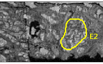
Let’s now compare two models, the biexponential and monoexponential decay models, with the value of the ΔAIC. Where these two models overlap, namely when the amplitude of one component is zero and the decay components are equal, the two models fit equally. In this case, there is no difference in the RSS values of the two fits, and so RSSx/RSSy = 1. When this happens, the logarithmic term becomes zero, so the value of 2(kx – ky) is equal to two times the difference in the number of parameters or four. This means that at the meeting point of the two models, the monoexponential model is favored by a difference in AIC of four. Another way of putting it – the AIC is already biased toward selecting the simpler model in this case, meaning the decision boundary is different in our theoretical boundary versus what the AIC chooses. Returning back to my previous Part 2 blog post, I can fit a similar sample of my data shown in that post to compare how the AIC selects between the two models. The results are shown in the image below (Figure 57 in my thesis)
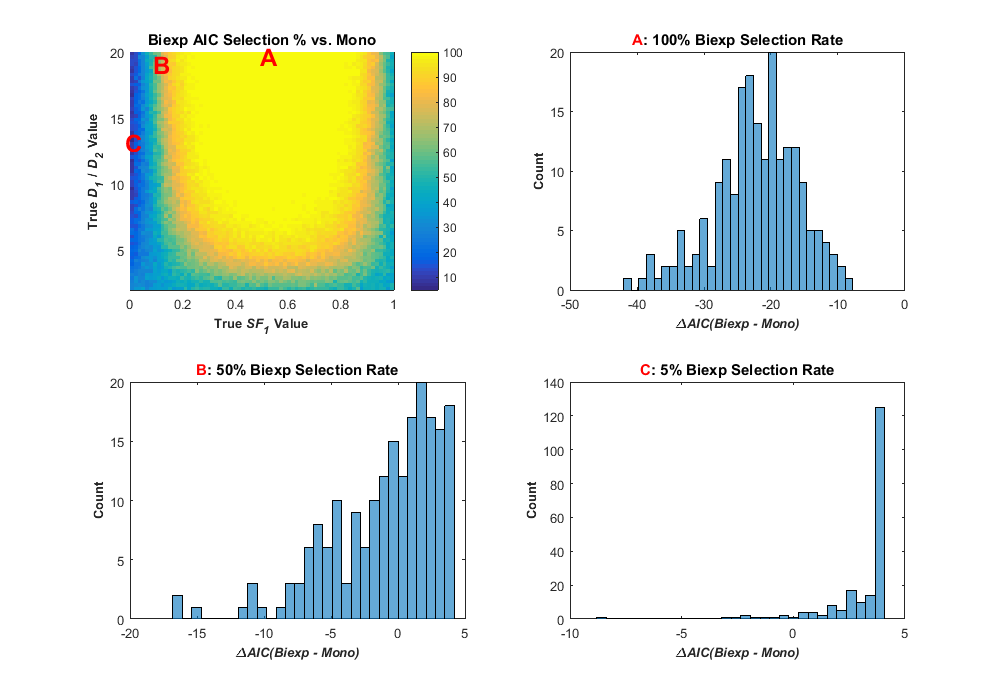
This figure has four plots. The top left shows a similar pseudocolor plot to my previous posts only the color refers to the percentage of simulated data in each point bin where the biexponential model was selected by the AIC as best. As you can see, where the signal is more distinctly biexponential (signal A, for example), the biexponential model is selected more. At the bottom and sides of the plot, where the true signal is closer to a monoexponential model, the monoexponential model was selected for many data points, and this monoexponential selection rate increased as the signal became more mononexponential (simulated SNR was 25 in this case). This plot shows the effect of the inherent bias in the AIC such that for some signals (signal C, for example), the monoexponential model was selected for 95% of the data based on that signal. The other three histogram plots show the distribution of the ΔAIC values for the the three sample signals A,B, and C. These histograms are interesting in that they show that even when the biexponential model was selected for all data from that signal, the spread is ΔAIC values is nearly 30. Thus, the difference in AIC values between the two models can vary considerably. There are many plots in Chapter 4 of my thesis related to model selection of simulated data, and you can check that out, if you really want to. One thing I found interesting, even if the simulated SNR in the data is increased to 200, the spread in ΔAIC values when comparing two models remains about the same (around 30). In retrospect, it isn’t totally surprising, since the closeness of fit of the two models, RSS, manifests in the equation as a logarithmic term. So, while the biexponential model was selected for more of the test data, there is still a boundary where the monoexponential model was selected for at least half of the signal data (see Figure 60 in my thesis, if interested).
AIC vs. Statistical Tests
While reading Burnham and Anderson’s book, you will run into the authors adamantly state that information-theoretic criteria are definitely not statistical tests. The distinction is made there and the authors recommend avoiding statistical testing, the p-value, and the declaration of significance. While doing my research, I came across a very interesting paper by Paul Murtaugh called “In defense of p-values”. In this paper, Murtaugh demonstrates similarities in performance of the p-value and the AIC. Murtaugh does a great job in addressing how the p-value acts just like the ΔAIC in that it breaks ties when two models have similar selection rates for a set of data. It’s a really nice paper to read, if you are interested in model selection, and it does a good job at harmoniously bridging statistical tests and information-theoretic criteria. Interestingly, in the same journal issue Burnham and Anderson have a commentary on Murtaugh’s paper called “p-values are only and index to evidence: 20th vs. 21st century statistical science”. I’ve now re-read this paper several times, and from an argument standpoint, it seems like Burnham and Anderson’s point here is that statistical tests are “so last century”, hence they shouldn’t be used. Instead “space-age” information-theoretic criteria are de rigueur in today’s science.
In retrospect, it’s rather strange that Burnham and Anderson seem quite hostile to Murtaugh, given that Murtaugh was trying to show how we can all get along. Also in retrospect, after being in academia for several years, I would expect nothing less. I started reading Prof. Deborah Mayo’s blog, Error Statistics Philosophy during the course of my PhD research, and found the discussions there quite informative and interesting, even though the philosophical rigor in a lot of the arguments goes over my head. The two blog posts on Murtaugh’s paper and Burham and Anderson’s paper are quite interesting, especially when reading the comments. See here for one from 2014 and here for a later one from 2016. You might get an idea from those posts on what the statistical debate is all about. Since this whole debate was fascinating, I compared the AIC and the statistical F-test in my data simulations, along with the AICc, which is the corrected version of the AIC. What I found can be seen in the image below.
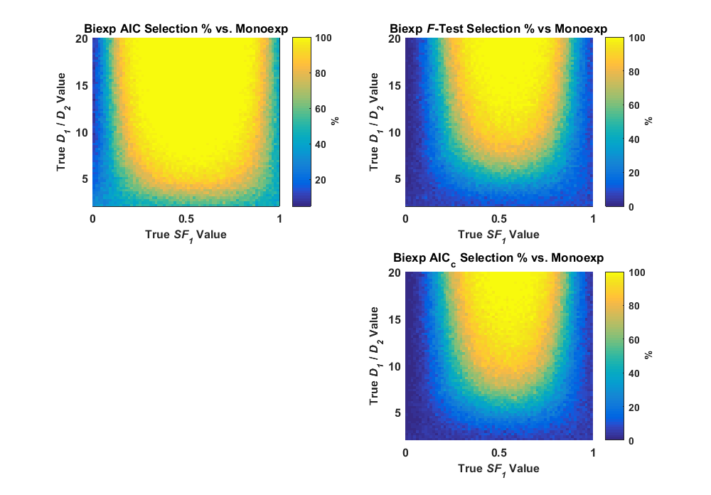
Here, my simulations show that the F-test (significance level α = 0.05) selects the simpler monoexponential model even more often than the AIC, and that the selection rates are nearly identical to the AICc. Thus, the p-value in the F-test does what it’s supposed to do, breaks ties by setting its decision level to the tail of the distribution (5%) as opposed to the center of the distribution (50%). The corrected version of the AIC also performs the same thing, although I only tested a small data sample representing a simulated voxel with eleven measurements. While I’m not a statistical philosopher, I was pleased to see these simulated tests show that these three statistical methods all select a model in very much the same fashion. No one model selection method is more “accurate” or “reliable” than another and, some methods simply select a more complex model at a more conservative rate.
Why the fuss?
If some model selection methods select differently than others, then why fuss over the differences? It’s great to know how the methods work when the truth is known in simulation, but what should I do for my data? I show in my thesis that the AIC selected similar to cross-validiation when comparing a few models. If you are in the machine learning world with tons of data, cross-validation is still the gold standard, especially if your data set is large enough to create multiple training/test set combinations. Often, even cross-validation might only show that one model is a slight improvement over another. For situations where we might have millions of data points, a 1 – 2 % improvement could be very valuable, for example, if those data points translate into a cost or speed efficiency. In the diffusion MRI literature, model selection is often used as an additional source of evidence that one model is preferred over another. However, remember that model selection methods are usually based around how well the model fits the data. The AIC is no different, as it uses the RSS value from the regression fit, and thus I should probably restate the concept again in this post:
If a model fits a data set better than another, that doesn’t mean that its parameter estimates are more accurate.
I show how this is the case near the end of Chapter 4 in my thesis, where I looked at a sample measurement where the AIC gave near-equal scores for the biexponential model and monoexponential model. For this fit, the biexponential model parameters have high uncertainty and are far from the true values. This is probably obvious if you’ve read my posts thus far, since the above plot of where the AIC selects the biexponential model looks very similar to the parameter uncertainty plots in my previous posts. While it would be nice if the AIC could help us avoid monoexponential-like signals where the uncertainty is high in the biexponential model parameter estimates, that is unfortunately not the case. However, using simulated data in Chapter 4 and actual data in Chapter 5, I show that if you use a minimum ΔAIC of 10 for using the biexponential and kurtosis models’ estimates, the uncertainty in the estimates decrease.
One last thing regarding AIC and model selection, in their book Burnham and Anderson talk about how AIC can be used to average parameter estimates across multiple models. I was very interested in doing something like this to create “meta-parameters” to gain more information about a model. After doing this model selection work, I came to the conclusion that this could be very dangerous with the biexponential and kurtosis models, since ill-conditioning can affect their parameter estimates and the AIC is not precise enough to avoid ill-conditioned fits. In the 2016 post above in the Error Statistics blog, Brian Cade comments that this multimodel averaging can be dangerous when multicollinearity is involved. A link to his 2015 paper, “Model averaging and muddled multimodel inferences” is found there, and I found it very interesting that he had already came to the same conclusion. His paper is a much more thorough and rigorous treatment of the subject, and I recommend it.
At the End
Looking back now, it’s interesting to think of the summary I would give about my PhD research. At the start, I was reading to crank out evidence of more complex models producing better results on all kinds of data sets. Certainties! Certainties! Certainties! After doing all of my simulation studies, I’m glad things turned out the way they did and am happy to live in our universe of uncertainty. Although sometimes we are forced to make a decision between one method or another, it often makes sense to be able to change one’s mind at a moment’s notice. In retrospect, this is how science and engineering improve. We create a model, we throw data at it, and we improve that model. Sometimes, we run into edge cases or outlier values where the model suddenly breaks down. It is at these edges where we improve our knowledge. We should always be asking the question, how would my results change under different circumstances? These circumstances could include different data, equipment, statistical measures, machine learning algorithms, selection criteria, prior distributions, hyperparameters, etc. I’m now using this philosophy in my work on machine learning, algorithms, and software development, and have a real passion for uncertainty and not only the way things work, but how they break