Part 2: The Biexponential Model and Ill-Conditioning

This post is the second one I am making in a series of posts based on chapters in my PhD thesis. The first one is here, the third one is here, and the fourth one is here

In my introductory post, I discussed the concept of a mathematical model and introduced the single exponential decay model that assesses that Apparent Diffusion Coefficient (ADC). This model is now a clinical standard, but many researchers feel that it is too simplistic. With improvements in MRI technology and machines that have higher signal-to-noise ratio (SNR), more features in the human body are now able to be accurately assessed. This had led to the development and testing of newer, more complex models that accommodate these features and provide more information. As I mentioned in my previous post, one of these more complex models in the biexponential model – a sum of two individual exponential decay components:

S = A₁ exp(-bD₁) + A₂ exp(-bD₂)

I’ve changed the variable names slightly here from the equation I used for the monoexponential model. Instead of a ratio of S to S₀, the amplitude components of the signal have shifted to the right side of the equation and have changed to A₁ and A₂, and are the individual signal values of each component at b = 0. You also might have noticed that I’ve changed the diffusion coefficients in each term from ADC to D₁ and D₂. These two diffusion coefficients are still apparent coefficients because in human tissue measurements they aren’t actually assessing Gaussian distributions, but I changed the terminology to distinguish them from the monoexponential term ADC. This biexponential model was used nearly 30 years ago in a live patient measurement (known as in vivo) of the brain to assess two separate components in each discrete volume, a diffusion component due to water moving within the cellular structure and a perfusion component due to blood flowing in vessels and capillaries. When assessing live human tissue, because perfusion moves the blood during the time period of the scan, its diffusion coefficient will be much higher than the diffusion component and the faster component is usually presented as component 1. This model has four separate parameters (A₁, A₂, D₁, and D₂), providing more information than the two-component, monoexponential model. The biexponential model is often seen in a slightly different form:

S = A₀ [SF₁ exp(-bD₁) + (1 - SF₁) exp(-bD₂)]

In this form, the two amplitude components have been split into a form where A₀ equals the amplitude at b = 0 (note: A₀ = A₁ + A₂), and a component SF₁ which represents the normalized signal fraction of each component. In this manner, the signal fraction can be used to assess how much each component contributes to the overall signal. For example, a value of SF₁ = 0.3 means the faster perfusion component “1” contributes 30% to the overall signal, and the diffusion component contributes 70% to the overall signal. This is then often interpreted in the literature as a volume fraction, such that in the measured volume, 70% is made up of tissue that diffuses and 30% of blood vessels and capillaries. This gives the capabilities to not only assess two separate diffusion coefficients, but how much each of these diffusion coefficients contribute to the overall signal. This biexponential model has been used in thousands of these sort of assessments in the diffusion MRI literature, with new research papers on it coming out every week. When specifically assessing in vivo data, this model is sometimes referred to as the Intravoxel Incoherent Motion (IVIM) model (see the paper in the previous paragraph for an explanation).

Biexponential Model Simulation

The very first project I worked on when starting my PhD research in 2012 was a simulation based on this biexponential model. This simulation was a project started by my supervisor and two other colleagues based on a comment made by a reviewer on one of my supervisor’s papers. This comment was really an age old question – for a given measurement, how do we know whether we are measuring signal or noise? For a single measurement, if we know that there is noise affecting our measurement process, then we don’t know what the true underlying signal is. If we know about how much noise is affecting our measurement, we can estimate a range that the true signal is likely to be in, but no amount of statistical magic can determine the true value from one single measurement. Thus, we often take several sample measurements to get a better idea. We can sample more measurements from the same volume (also known as a voxel in MRI – a 3D pixel) to get a more precise estimate of a given parameter. However, what is often done in many MRI tissue measurements is a grouping of many voxels in a region. After an MRI scan is performed, and a suspected malignancy is excised from a patient, this tissue is often sliced and scanned and a pathological analysis performed. If a pathologist looks at a slice of tissue on a slide and identifies a region of cancerous tissue, say, versus normal tissue, we can often go back to our MRI analysis and visually identify approximately the same regions on our MRI images.

This creates extra uncertainty in our analysis, for example our MRI and pathology images won’t exactly match up due to the changes in tissue after it is removed from the patient. We can use image registration techniques to better align our images, however, this still adds some additional noise to our analysis. Once we have two regions (normal tissue vs. cancer), we can group the voxels in each of the two regions and combine the model parameters for these voxels. This will give us two unique parameter distributions, upon which statistical analysis is often performed. This is how the monoexponential ADC parameter was identified to be lower in cancerous tissue vs. normal tissue, and this is often how most biexponential model analysis is performed. For example, the SF₁ parameter might be shown in a certain tissue condition to have a lower mean value in this region vs. a region without that anomaly. This type of analysis is often accompanied by a statistical test that demonstrates a significant difference in one or more parameters, emphasizing that this model is likely to be a good candidate for a diagnostic test.

If the biexponential model has been around for 30 years, then why isn’t it in widespread clinical use as a diagnostic tool? While, statistical analyses of model parameters are nice in their demonstration of differences between two regions, using statistics reduces the information in the analysis to a simple mean, standard deviation, or test of significance. This may mask the level of uncertainty in the model parameters, the heterogeneity in tissue differences, or what the model parameter images look like when displayed. If we are to use newer models as a part of clinical diagnosis, then these models should produce parameter maps that are of a high standard that radiologists can use. Yet, this doesn’t appear to still be the case for the biexponential model. This was noted in a 2016 review paper by Taouli et al that reported that when displayed as images, estimates of the perfusion/pseudodiffusion parameter were too unreliable to be used for diagnosis. Additionally, this review specifically noted that combining parameter data as distributions underestimates the errors in voxelwise estimation and concludes the biexponential model report by stating, “Data showing superiority of IVIM parameters over ADC for tissue characterization is limited, and more evidence is needed. IVIM parameter reproducibility and the role of IVIM parameters in treatment response need also to be better defined.”

The purpose of performing biexponential model simulations was an attempt to investigate why some of these parameters are so noisy and to diagnose how and why the uncertainty in these parameter estimates becomes so high under certain conditions. While a computer simulation can’t replicate real conditions in a tissue measurement, it can simulate thousands of measurements in seconds, a feat that would be very costly in terms of time and money with real MRI data. Additionally, with a computer simulation, the true conditions can be set and are known, such that the estimates can be compared to the true values in the analysis. This also eliminates the heterogeneity found when combining voxels in a region, meaning the variability in the parameter estimates comes solely from that due to the simulated noise. Thus, in my first submitted paper, we did just that. We used the second model equation presented above, and created a simulated test set. We set A₀ and D₁ to a normalized value of 1, and then created 50,000 parameter combinations where SF₁ was randomly chosen between 0 and 1 and the value of D₂ was randomly chosen between 0.05 and 0.5. We then selected 11 simulated b-values/diffusion weightings to create 50,000 noise-free signals. To each of these signals, simulated, random noise was added to represent the MRI measurement process and noise was added at SNR levels of 25, 100, and 200, with 200 noisy signals created at each SNR. This created a large test data set of millions of noisy sample measurements. For each of these measurements, the biexponential model was fit using a Nonlinear Least Squares (NLLS) fitting algorithm, and the parameter estimates were combined across the measurement fits for each noise-free signal. When the parameter estimates were plotted based on the noise-free signal measurements, the results looked like this (sample of SF₁)

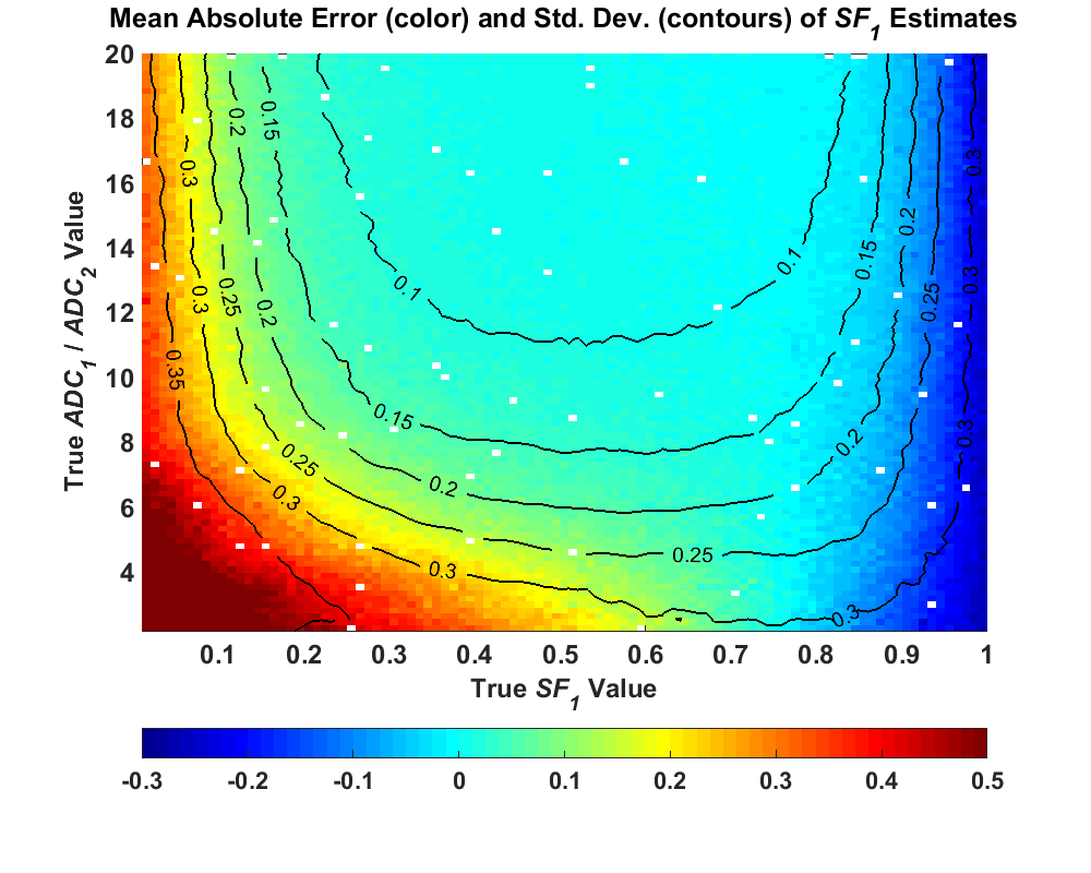
This image was sampled from Figure 10 in my thesis, and the rest of the plots in that figure can be seen there. What the figure above shows is that the uncertainty in the parameter estimates changed considerably based on the true parameter values of the signals. For some parameter combinations, the uncertainty was low, but at other parameter values, the uncertainty spikes to a very high value and is much higher than the other signals. This high uncertainty occurs specifically when the true signal is close to monoexponential – the signal fraction of the faster component is close to either 0 or 1 (nearly all of one component), or the ratio of D₁ to D₂ is low. In our original paper submission, we demonstrated this anomaly and concluded that the noise affects the different components, and was attributed to the lack of adequate diffusion weightings covering each component and the bias incurred by the Rician distribution of MRI measurements. A paper was published in 2016 by Merisaari et al demonstrating these same ideas and coming to similar conclusions. This paper was more comprehensive than ours and included real data to back up their findings. Yet as I noted in my thesis, the authors in this attribute the overestimated bias in the biexponential parameter values to the effects of the Rician signal bias and attribute most of the uncertainty to noise. Over the course of my PhD study, I slowly came to a different conclusion, and I’ll now spend some time attempting to convince you that there is another factor at work here.

Correlation, Collinearity, Conditioning

I’ll now shift from the world of medical imaging to a simple thought experiment using a favorite conceptual tool from the world of statistics education – urns with small, colored balls. Yes, this may seem silly, but bear with me - there’s a point here somewhere. Imagine that we have a room with two large urns with thousands of balls each, and one urn has all white balls and the other black balls. Let’s also say that these two urns are in a room where, unbeknownst to you, a friend of yours flips a coin 20 times and if this coin comes up heads, he/she puts a black ball in a separate bowl, and if the coin comes up tails, he/she puts a white ball. You then come into the room and your friend asks you to guess how many balls came from the black ball urn and how many came from the white ball urn. This seems rather trivial, you count the number of balls in the bowl and you see, let’s say, 12 black balls from the urn with black balls and 8 from the urn with white. You then look at the two urns and quickly conclude that 12 balls came from the black ball urn and 8 from the white ball urn…and you would be correct. This would probably seem obvious and silly, and a part of you would probably think that this some sort of elaborate ruse. Now you leave the room and let’s say that the urn with all white balls is replaced by another urn with thousands of black balls that are identical in every way to the first urn. Your friend now randomly selects 20 balls per the coin flip method and you come back in the room. Your friend again asks you to guess how many balls came from each urn. You now really feel that this is an elaborate ruse.

If all of these balls are identical, how are you supposed to know what urn they came from? There is no way to tell them apart! So, you’d probably make a guess because you have a 1/21 chance of getting it right (the true value would be any integer from 0-20 for the balls coming from the first urn). That’s just under 5% odds of getting the value by chance alone (smells like significance again). However, if there were a total of 2000 balls being drawn, the odds of getting the exact value drop dramatically. This seems like a silly scenario because it seems so obvious that this is pointless – the only way to get it right is to guess. My point of these scenarios was to illustrate why inverse problems are so much more difficult in nature. Your friend was in charge of the “forward” problem: select twenty random balls to create a data “set”. He/she has the information of how many balls came from each urn. You come into the problem with no knowledge or information about the balls, so you rely only on the information at hand. If the balls in each urn are easily distinguishable, then the problem is absurdly easy. If there balls are identical, then there is no way to distinguish between the two balls and the problem is absurdly hard (and impossible). Getting the right answer in this case is due solely to chance.

We can compare this problem to the mathematical concept of correlation. We usually see correlation in scientific and statistical practice as a measure of whether one factor depends on another. So, let’s say we are conducting an experiment, and an increase or decrease of one factor leads to the same increase or decrease in another. We might then conclude that there seems to be some relationship here that is worth pursuing. For example, let’s say we have a hypothetical study that shows that there is a correlation in humans between increased consumption in drinking coffee and increase in incidence of cancer. Our natural response is to think that if we cut our coffee consumption then our chance of getting cancer in our lifetime would be reduced, right? This is where the maxim of “correlation does not imply causation” comes into play. Just because there is a correlative relationship doesn’t automatically mean that “coffee causes cancer”. There are so many other factors that affect humans over the course of a lifetime, that we can’t isolate coffee drinking as a single factor. Genetics, exercise, obesity, dietary habits, etc. could all affect rates of cancer incidence.

In this dependence relationship between two factors, a high correlation (Pearson’s coefficient ρ -> 1) is usually desirable in a study, but let’s look at a different correlative relationship. Using this same hypothetical coffee/cancer relationship, imagine we have a sample population, and in addition to recording cancer incidence and coffee consumption, we also record tea consumption. If we analyze our population data, let’s say that we find that coffee consumption and tea consumption are perfectly correlated (ρ = 1). From this data we also see a high correlation between cancer incidence and coffee consumption. Because coffee and tea consumption are perfectly correlated, we would see this exact correlation between cancer incidence and tea consumption. However, if we wanted to distinguish whether coffee consumption OR tea consumption was correlated with cancer incidence, we are faced with the same problem as when confronted with sampling from two urns of identically colored balls. Because, these two factors are perfectly correlated independent variables, there is no way to separate their effects on the dependent variable and this inverse problem is, for practical purposes, impossible. We would need to repeat a study where the correlation between coffee and tea consumption is much lower.

We will now shift this same concept into the world of mathematical modeling. Let’s say that we want to model this mathematical relationship of coffee consumption and tea consumption versus cancer incidence as a simple linear relationship. We will let y be cancer incidence, x_c as coffee consumption, and x_t as tea consumption, with a model equation of

y = x_c + x_t

If we then performed a linear regression with our previous patient data set using this equation, we would assign two β parameters to be the regression coefficients, representing the contribution of each individual independent variable to the dependent variable:

y = β_c x_c + β_t x_t

We would then enter all of our data into our linear regression algorithm and let the algorithm solve for the two β parameters. However, let’s analyze what would happen if tea consumption and coffee consumption are perfectly correlated. If this is true, then in our model equation x_c = x_t. We could set these two variables to just x, which, after combining factors, gives us the equation:

y = (β_c + β_t) x

This poses a problem in our analysis. Let’s say that we only compared coffee consumption using the model equation y = β_c x_c and after performing a linear regression on our data, we get a value for β_c of 1. Because coffee consumption and tea consumption are perfectly correlated, in our combined and refactored model equation, we are attempting to solve the equation

(β_c + β_t) = 1

This is what is known in linear algebra as an underdetermined system in that there are fewer equations than unknown variables. In this case, we can think of an infinite number of combinations that could solve this equation (e.g. (0.1, 0.9), (0.5, 0.5), (-99, 100)). This demonstrates how attempting to separate these perfectly correlated, independent factors is also mathematically difficult. These types of problems are also called ill-posed. When we our independent factors are perfectly correlated in a linear system like this, we also say that these factors are perfectly collinear. For most data, however, we don’t have perfect collinearity, and we don’t know the extent it may be affecting the parameter estimates. Furthermore, typical regression quality measures are based only on how well the model fits the data, and are inadequate in detecting collinear parameters. For example, if the two independent variables are perfectly correlated, then their effects on the dependent variable would be the same. So, if we looked at the combined model equation and how well it fit our data

y = β_c x_c + β_t x_t

and compared that to how well a single factor fits the data

y = β_c x_c

using conventional goodness-of-fit measures such as RSS or R², these two models would fit exactly the same. Thus diagnosing collinearity requires extra detection measures. One of these measures in linear regression is the condition number of the matrix calculated in the regression algorithm. This condition number indicates the sensitivity of the output of the equation to changes in the input. In a well-conditioned problem, small changes in the input values result in small changes in the output. In an ill-conditioned problem, small changes in the input values can result in large changes in the output, or vice versa. Thus, while the model equation above with the two correlated factors would fit the data identically as the single factor model, the values of the parameters would be highly sensitive to changes in the data. Any noise in the data would be amplified in the parameter estimates, producing highly uncertain (unstable?) results. This illustrates why relying solely on goodness-of-fit measures can be dangerous as a measure of whether one model should be preferred over another.

Ill-Conditioning

After that conceptual detour, we’ll now return back to the subject of interest in this post, the nonlinear biexponential model. Looking at its model equation again

S = A₁ exp(-bD₁) + A₂ exp(-bD₂)

we can now see that a similar effect can occur in this model. If D₁ = D₂ then we can reduce the above model equation to the variable D

S = (A₁ + A₂) exp(-bD)

This again is an underdetermined system where there can be an infinite number of possible values for A₁ and A₂. Additionally when fitting a monoexponential signal, the biexponential model equation can be viewed as a model equation with a redundant decay component and two redundant variables A₂ and D₂ which are no longer identifiable because they don’t exist in the signal. While the biexponential model has been in use with diffusion MRI applications for nearly 30 years, problems with using this model in data fitting have been known about for much longer. In his 1956 book, Applied Analysis, Cornelius Lanczos gave a well-known example that demonstrates how a three-term (triexponential) exponential decay model equally fits a certain set of data such that there are many possibilities for parameter values that may be returned by a fitting algorithm. Forman Acton put it much more bluntly in his 1970 book Numerical Methods that Work:

“For it is well known that an exponential equation of this type in which all four parameters are to be fitted is extremely ill conditioned. That is, there are many combinations of that will fit most exact data quite well indeed (will you believe four significant figures?) and when experimental noise is thrown into the pot, the entire operation becomes hopeless.”

This is exactly what we are doing when fitting diffusion MRI data with this model, since there is experimental noise added to our measurements. Why have these problems not been discussed before in this field? As I discussed previously in this post there is a lot of heterogeneity in most real diffusion MRI data, such that problems with the fitting method may be masked by differences in the tissue being measured. Additionally, publishing analysis results using a mean and standard deviation, as noted earlier, also masks the distribution of the results. So, what exactly were the results of fitting my data simulations? The pseudocolor plot I showed above demonstrated that there was considerable bias and variance in the fitted parameter estimates, and that this bias and variance changed based on the true parameter values. As I also noted the bias and variance becomes more extreme when the true signal is closer to a monoexponential signal, either due to very little signal from one component or a low ratio between the two diffusion coefficients. After now showing how ill-conditioning can conceptually occur in the biexponential model, these simulation results show that ill-conditioning may indeed play a part in the uncertainty found in the parameter estimates. I came to this conclusion due to the uncertainty in the parameter estimates being much larger than the uncertainty from the added simulated measurement noise. Additionally, when the simulated SNR is increased, there were more signals that could be reliably fit with the biexponential model, but signals that were effectively monoexponential model. What do I mean by reliably fit? I will show some histograms in a plot from my thesis (Figure 12). The simulated noise added to the true signal was, for most data points, effectively Gaussian. When examining how the monoexponential model was fit to my data, the parameter estimates from simulated noisy data from one true signals had a distribution that was effectively normal centered around the true value. The results from the biexponential model, however, changed depending on what the true value was. Looking at signals where the ratio between the two diffusion coefficients was 8, 4, and 2 a noticeable degradation of the estimates can be seen as the ratio decreases (becomes more monoexponential)

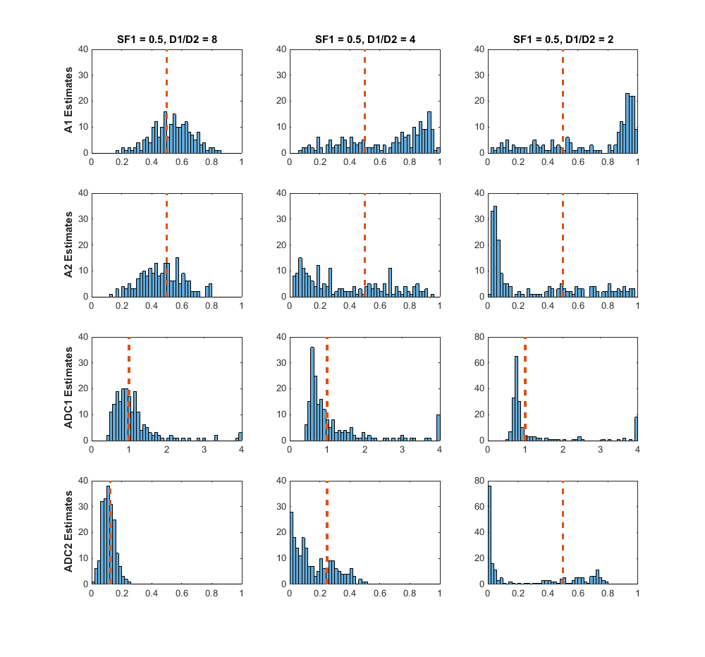
For the ratio-of-2 signal, aside from the majority of parameter estimates clustered around a value that is not the true estimate value, there are many estimates that are widely dispersed and found at several orders of magnitude above or below the true parameter value. Thus, I concluded from this that the reliability of the biexponential model can be questioned when measuring certain signals, and it should be used in data analysis with extreme caution.

But this doesn’t apply to the real world!

This was effectively the critique that led to the rejection of our initial paper submission and was also a critique from the reviewers of my PhD thesis. To me, these sorts of comments can feel something like, “Hey, we are in the real world here. These computer simulations are cute and all, but we are in the serious business of medical imaging diagnosis. Produce results that support actual data.” And so, during the course of my PhD, and in the time since, papers, posters, and talks keep getting published using this biexponential model. Because what is important is the story, the data, the results, and the paper. Whether or not the software is producing reliable results is an afterthought. However, while working on my analysis of the biexponential model, I did a thorough study of ways to diagnose issues when fitting data, came up with an effective method for assessing the uncertainty of the estimates of a single measurement, and applied this to real-world data in my thesis. This will be the topic of my next blog post, along with a visualization of the NLLS regression fitting problem, and a short analysis of fitting data with another diffusion mri model known as the kurtosis model.

Acknowledgements

I would like to specifically acknowledge the contributions of my co-authors on the initial, rejected paper I discussed, which ultimately led to the bulk of the material of my PhD thesis. Thanks to Dr. Roger Bourne, Prof. Zdenka Kuncic, and Dr. Peter Dobrohotoff.