Nonlinear Regression Primer
My first task as a new PhD student was to investigate why a particular Monte Carlo simulation was having problems. The simulation involved fitting simulated noisy signals with a biexponential model using a Nonlinear Least Squares (NLLS) regression algorithm in MATLAB. I started out knowing hardly anything about least squares regression, linear or nonlinear, but slowly figured things out along the way. At first I was interested in solely getting the desired parameters from the algorithm, but after I spent a lot of time stepping through MATLAB’s various NLLS regression functions, mostly lsqcurvefit, I learned a lot about how these algorithms work and how to diagnose issues with nonlinear models used with them. For typical NLLS regression problems, you probably won’t be concerned with the inner workings of the algorithm, however, if you are using functions that may have trouble finding a global minimum or are interested in more information than the returned parameter values, such as estimated confidence intervals, this may help you out.
I wanted to write this post because I wasn’t able to find a lot of information on nonlinear regression algorithms starting out, other than put in your data and model here, get results there, and here are the various algorithms you use. Too easy, right? It’s also hard to find assistance on why you would care about this stuff that doesn’t usually involve a lot of math-heavy analysis. You’ll probably find that most of your books out there will get into linear least squares regression and discuss regularization, LASSO, Tikhonov, etc., but NLLS problems are usually addressed with only a few pages or often not at all. Thus, I ended up browsing the MATLAB function manuals, faced with all of these inputs and outputs and no real idea as to what they actually do. After spending six years in graduate school, I did find that I really like mathematics, but I learn concepts much better from reading and debugging computer code as opposed to mathematical notation. I still have trouble with it like I still have trouble reading sheet music. I found that understanding a difficult concept requires several different sources to fully grasp the meaning, so I will add books that helped me at the bottom of this post.
If you use MATLAB, I added the code examples here in one file, which is available on my github site here. I ran all code in MATLAB version 2015a. Python has good scientific and statistical libraries, and more importantly, it’s free, so I’ll try and create a similar Jupyter notebook at some point. If you use R, I highly recommend the book, Nonlinear Parameter Optimization Using R Tools by John C. Nash. It’s fairly new (2014) and his explanations and walkthroughs of NLLS regression problems in Chapter 6 are extremely valuable even if you don’t program in R. He actually has written his own R packages for nonlinear regression and optimization problems, he explains details like Jacobians and gradients, and most importantly, there are tons of code examples. I used some of his packages to compare my MATLAB results.
What does nonlinear regression look like?
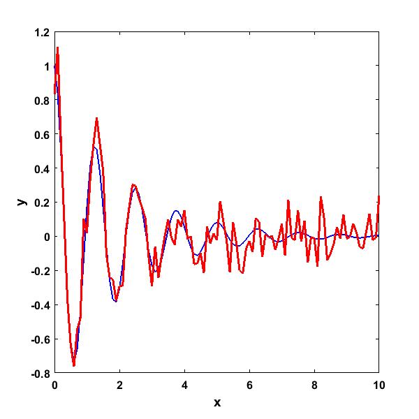
A good place to start with when using NLLS regression problems is to plot our data. This is always a good idea when performing any sort of exploratory analysis on data, and the importance of this is illustrated here. For the sample data on this page, I created a simple set of data using the model function
y = exp(-β1∙x)∙cos(β2∙x) + ε
To create noisy data, an array of data for x was created, with β1 and β2 set to 0.5 and 5 respectively. At each data point, normally distributed random noise with a standard deviation of 0.1 was added (ε).
x = 0:0.1:10;
beta1 = 0.5;
beta2 = 5;
NumParams = 2; % Number of model parameters
stdnoise = 0.1;

y = exp(-beta1.*x).*cos(beta2.*x);
ynoise = y;
for i = 1:length(x)
	ynoise(i) = y(i) + stdnoise*randn(1);
end
Producing this plot where the blue line is the original signal and the red line the signal with added noise
Given this noisy signal, we’d like to use a regression algorithm to now estimate the value of the two original β parameters. As you can see in the formula, these parameters both have a nonlinear relationship to the dependent variable y, so a nonlinear regression algorithm needs to be used. In this example, we will use MATLAB’s lsqcurvefit function. We’ll walk through the code and then explain all of the inputs and outputs. First, we will declare the options:
FitOptions = optimset('Display', 'iter-detailed', 'Algorithm', 'levenberg-marquardt');
The ‘iter-detailed’ option will return a detailed output of how the algorithm searches. Because it’s a nonlinear regression algorithm, initial starting values of both β parameters must be provided. This is because the NLLS algorithm is doing a linear approximation of the values and not calculating an exact solution (more here). We’ll use (1,1).
StartGuess = [1,1];
Now, we need to code our formula above (note, where and how this function is declared may affect whether the code runs).
function signal = DecayCosine(p, x)
signal = exp(-p(1).*x).*cos(p(2).*x);
And finally, run the regression algorithm. Note, we aren’t putting any lower or upper bounds on the parameter values in this case, hence the empty arrays ([]).
[RetParams,RSS,Residuals,ExitFlag,Output,RetLamb,RetJacob] = lsqcurvefit(@DecayCosine, StartGuess, x, ynoise, [], [], FitOptions);
After the function finishes, the variable RetParams contains the values of the two β parameters.
RetParams =
    0.4854    5.0016
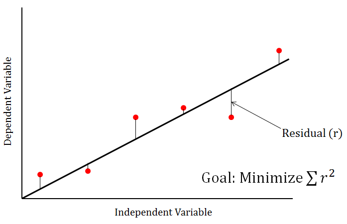
This shows that after the addition of noise, the best parameter estimates aren’t quite the same as the original values of 0.5 and 5, but are fairly close. The next two values in the returned parameter array are the variables RSS and Residuals. These two values are related - the RSS is also known as the Residual Sum of Squares, which is the sum of all squared residual values. In our particular fit, the Residuals array contains all 101 residual values. At each data point, the residual is the remaining vertical distance between the original data point and the value of the line/curve of best fit. Here’s a simple graph with a line of best fit to illustrate
As part of diagnosing a regression fit, it can be important to sometimes look at the distribution of the residuals.
figure('Position', [50,50,600,600]);
histogram(Residuals,25); xlim([-0.4 0.4]);
xlabel('Residual Distance','FontWeight','bold','fontsize', 14); % x axis label
ylabel('Count','FontWeight','bold','fontsize', 14); % y axis label
set(gca,'FontSize',12,'FontWeight','bold'); % Fix axis label font size

With these residuals, it’s hard to determine whether these residuals are exactly normally distributed, but the histogram is a well-formed distribution and normal-like. The value of RSS is then the sum of each of these residual values squared. As the residual line plot above shows, the RSS is the value that the algorithm attempts to minimize. Let’s look at the returned display after running the algorithm
                                        First-Order                    Norm of
 Iteration  Func-count    Residual       optimality      Lambda           step
     0           3         9.31579            1.67         0.01
     1           6         6.45792           0.358        0.001        1.71525
     2           9         5.57083          0.0242       0.0001        3.95479
     3          14         5.20695           0.123         0.01        3.03434
     4          18         4.84218           0.213          0.1        1.12208
     5          21         3.50569           0.661         0.01         1.7379
     6          26         2.60861            1.02            1       0.542149
     7          29         1.19341           0.967          0.1       0.605667
     8          32         1.07528           0.739         0.01       0.177536
     9          35         1.04302          0.0381        0.001      0.0501656
    10          38         1.04291         0.00634       0.0001     0.00356785
    11          41         1.04291        0.000995        1e-05     0.00058131
    12          44         1.04291        0.000157        1e-06    9.14717e-05

Optimization stopped because the relative sum of squares (r) is changing
by less than options.TolFun = 1.000000e-06.

Optimization Metric                                  Options
relative change r =   7.35e-08              TolFun =   1e-06 (default)
The algorithm runs through successive iterations as part of its attempt to find the minimum value of RSS (shown as Residual in the table). The output shows that it took 44 function calculations to find the minimum value. The algorithm also reported that the difference in function between the last two steps was less than 1e-6. This means the algorithm appeared to have found a minimum as the neighboring fit points have minimal difference in RSS values. How the algorithm found this particular minimum can be plotted as a 3D contour graph.
% Calculate the RSS values in the neighborhood of the parameter values
Beta1Range = 0:0.05:5;
Beta2Range = 0:0.1:10;
RSSForParams = zeros(length(Beta1Range),length(Beta2Range));

for i = 1:length(Beta1Range)
    for j = 1:length(Beta2Range)
        Params = [Beta1Range(i), Beta2Range(j)];
        RSSForParams(i,j) = CompareRSSOfTwoSignals(DecayCosine(Params,x),ynoise);
    end
end

% Plot a 3D contour of the RSS values
figure('Position', [50,50,700,600]);
% whitebg('k'); % if you want to set the background to black for contrast
colormap('jet'); % change the default color map for contrast
contour3(Beta2Range,Beta1Range,squeeze(RSSForParams(:,:)),0:0.025:20); % 3D contour plot
zlim([0 20]); % Set the z dimension range to match the contour plot values
xlabel('\beta2','FontWeight','bold','fontsize', 14); % x axis label
ylabel('\beta1','FontWeight','bold','fontsize', 14); % y axis label
zlabel('RSS Value','FontWeight','bold','fontsize', 14); % z axis label
set(gca,'FontSize',12,'FontWeight','bold'); % Fix axis label font size
HandleC =  colorbar('location', 'EastOutside');
HandleCLabel = ylabel(HandleC,'RSS','FontSize',14,'FontWeight','bold');
% Optional code to rotate the colorbar label 180 degrees
drawnow; % MUST STICK THIS HERE TO GET THE NEXT PARTS TO WORK
LabelPos = HandleCLabel.Position;
HandleCLabel.Rotation = -90;
HandleCLabel.Position = [LabelPos(1) + 1.1, LabelPos(2), LabelPos(3)];
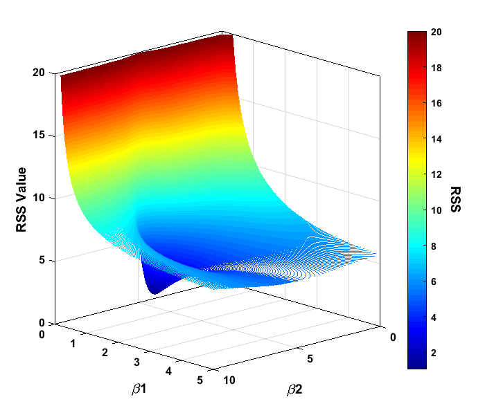
This plot was created by calculating the RSS value between the noisy signal and a 101x101 grid of discrete (β1,β2) combinations. To rotate the 3D contour plot to this angle, click the Rotate 3D button near the top of the figure window. When plotted as a contour, the “shape” of the regression problem can be seen with a very high value of RSS at β1 close to zero, and as the value of β1 increases, the RSS value decreases like a ramp and levels off. This makes sense, as the value of exp(-β1) decreases as β1 increases. In the center of this ramped surface, there is a 3D parabola shape in which the RSS value decreases even further. At the bottom of this shape is the minimum that was found at the (β1,β2) values of (0.4854, 5.0016), and yes, the entire shape looks kind of like this. The NLLS regression algorithm searches for this minimum, and does this by estimating the slope of the curve in the vicinity of the current location. If we add a position display line of code to our function algorithm
% Fit function
function signal = DecayCosine(p, x)
disp([p(1),p(2)]);
signal = exp(-p(1).*x).*cos(p(2).*x);
The current parameter values as the algorithm attempts to find the minimum can be seen. For our example above, if we look at the contour plot from above, we can plot out the path that the algorithm took to solve the problem. Note: I removed a few values in the plot where the algorithm tested points that were outside the displayed range of values.
% Note, the path went outside the above area, so I changed this line
% and re-ran the contour plot code above
Beta1Range = 0:0.05:7; % This changes for display purposes in this graph

% Now for the line plot
hold on;
plot(ParamPosArray(:,2),ParamPosArray(:,1),'k','LineWidth',1.5);
% Add the start (green) and end (red) points
scatter(ParamPosArray(1,2),ParamPosArray(1,1),'g','filled');
scatter(ParamPosArray(end,2),ParamPosArray(end,1),'r','filled');
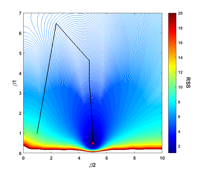
The plot shows the progress of the algorithm from it’s starting point of (β1,β2) = (1,1) to the minimum it found. We can also think of this as putting a marble at the starting point and letting it naturally roll to the bottom, akin to those plastic surfaces that let you roll coins into it for charity.
Our particular modeling problem was straightforward since we found what appeared to be the global minimum. For some nonlinear problems, algorithms can get caught up in local minima, which appear to be the best solution, but instead the algorithm is trapped and can’t get to the global minimum. This is why displaying a contour plot in the neighborhood of your solution can be helpful, as multiple minima can possibly be identified. There are also algorithms that do a more exhaustive search of the parameter space to find the global minimum such as simulated annealing or genetic algorithms among others.
Regression Error
We already saw that the RSS is the measure that the algorithm attempts to minimize, and this value is often used to test the goodness-of-fit of the model to the data. One measure that is often used in regression problems is R2, often called the coefficient-of-determination. The RSS can be also be used to compare various models using a statistical F-test or Akaike’s Information Criterion (AIC), for example. Model selection and goodness-of-fit is a topic in itself and I actually discuss it in my PhD Thesis. One measure that is often overlooked, but I like, is the Standard Error of Regression (SER). I like the SER as it can be related back to our regression problem equation
y = exp(-β1∙x)∙cos(β2∙x) + ε
In this problem equation, SER is the estimate of ε, the amount of noise in the equation. The SER is calculated using the formula
SER = sqrt(RSS/(n - p))
where n is the number of data measurements and p is the number of parameters in our model equation. The expression n-p is derived from the statistical degrees of freedom in our problem. If we use the RSS value from our fit above, we get
NumMeas = length(x) % number of data points
SER = sqrt(RSS/(NumMeas - NumParams))

SER =

    0.1026
Note that this SER value is very close to the standard deviation of the noise we added to our original data (0.1). This value is also related to the width or standard deviation of our residual distribution we saw earlier
std(Residuals)

ans =

    0.1018
Jacobian
Looking back at the lsqcurvefit algorithm, we can see that we’ve discussed the returned parameter values as well as the residuals and RSS. The ExitFlag tells you why the algorithm stopped and the Output provides a summary of information as to what the algorithm did during the search. The next output Lambda provides information about Lagrange Multipliers, which I personally do not have a lot of experience with. The last output is the Jacobian, a very useful matrix in NLLS regression problems. In our particular case, using the Jacobian matrix can help us do two things: speed up our algorithm to find the minimum and calculate diagnostic values for our parameter estimates.
I will oversimplify this here, but essentially the Jacobian is a matrix of the first-order partial derivatives. In our contour plot, the Jacobian is a local estimate of the slope of the surface at each iteration. In lsqcurvefit’s implementation of our particular algorithm, Levenberg-Marquardt, the Jacobian is estimated using finite differences. However, a user-defined Jacobian can be provided in the model function code to assist the algorithm with a more accurate Jacobian value. We’ll modify our DecayCosine model function with an added Jacobian and re-run the lsqcurvefit fitting code again. I manually calculated the individual Jacobian components using WolframAlpha as a quick way to do it. MATLAB has a symbolic toolbox that should let you calculate the derivatives within the function itself, but I had trouble getting it to work.
function [signal,jacobian] = DecayCosineWithJac(p, x)
signal = exp(-p(1).*x).*cos(p(2).*x);
% Create the Jacobian by calculating the derivative of the above function with respect to the individual parameters
JacobPt1 = -x.*exp(-p(1).*x).*cos(p(2).*x); % d/dp(1) or d/da(exp(-a*x)*cos(b*x))
JacobPt2 = -x.*exp(-p(1).*x).*sin(p(2).*x); % d/dp(2) or d/db(exp(-a*x)*cos(b*x))
jacobian = [JacobPt1' JacobPt2'];

% Modify the options to include user-provided Jacobian
FitOptions = optimset('Display', 'iter-detailed', 'Algorithm', 'levenberg-marquardt','Jacobian','on');

% Change the model function to our Jacobian one
[RetParams,RSS,Residuals,ExitFlag,Output,RetLamb,RetJacob] = ...
	lsqcurvefit(@DecayCosineWithJac, StartGuess, x, ynoise, [], [], FitOptions);
After running the algorithm using the function with our user-provided Jacobian, we get the same parameter estimates, (0.4854, 5.0016), however, look at how quickly the algorithm found the solution
                                        First-Order                    Norm of
 Iteration  Func-count    Residual       optimality      Lambda           step
     0           1         9.31579            1.67         0.01
     1           2         6.45792           0.358        0.001        1.71525
     2           3         5.57083          0.0242       0.0001        3.95479
     3           6         5.20695           0.123         0.01        3.03434
     4           8         4.84218           0.213          0.1        1.12208
     5           9         3.50569           0.661         0.01         1.7379
     6          12         2.60861            1.02            1       0.542149
     7          13         1.19341           0.967          0.1       0.605667
     8          14         1.07528           0.739         0.01       0.177535
     9          15         1.04302          0.0381        0.001      0.0501652
    10          16         1.04291         0.00634       0.0001     0.00356786
    11          17         1.04291        0.000995        1e-05    0.000581311
    12          18         1.04291        0.000157        1e-06    9.14718e-05

Optimization stopped because the relative sum of squares (r) is changing
by less than options.TolFun = 1.000000e-06.

Optimization Metric                                  Options
relative change r =   7.35e-08              TolFun =   1e-06 (default)
The number of function evaluations needed to find the solution was reduced from 44 to 18! This can be helpful if you need to use the algorithm thousands (or millions!) of a times on a large set of data.
Parameter Estimation
It’s probably a good time to look at our problem from a statistical inference perspective. What the NLLS algorithm attempts to provide is the most likely estimates of the model parameters given our set of data. The values of β1 and β2 that were estimated earlier are part of what is known as a point estimate - a single set of estimates from a set of measurement data from some underlying process. Often, however, we’d like to know what range of parameter values this process will likely produce in future measurements, for example, if we want to use this model for prediction or classification purposes. The best way of doing this is obviously acquiring more measurement data and examining the resulting parameters. This can be expensive and time consuming in many cases, for example, in in vivo MRI scans. It is possible, however, to obtain an interval estimate from a regression fit from one set of measurement data using the Jacobian matrix.
To obtain interval estimates, as well as other useful information related to the parameter estimates, we will start by getting the covariance matrix. The covariance matrix is returned as an output parameter if you happen to use MATLAB’s nlinfit or fitnlm functions. I will use custom code, instead, to calculate the covariance matrix from the Jacobian. If you are proficient with the MATLAB debugger, you can step through the code for nlinfit to find the section that calculates the covariance matrix. Rather than cause any copyright issues and get me in trouble with Mathworks, I will instead replicate code from a freely available MATLAB implementation of a variable projection NLLS algorithm by O’Leary and Rust. This code is an updated implementation of an older variable projection algorithm from the 70’s that was designed to obtain better estimates from difficult regression problems. You can read about the history of this algorithm and the new MATLAB code here (or as a published paper here), which gives a really good mathematical explanation of some of the parameter estimation values I will introduce here. I have used this VarPro code many times over the course of my PhD, and I will add some of my implementations to this site in the future.
The code for finding the covariance matrix from the Jacobian matrix has some matrix operations which I comment on below.
% The Jacobian returned by lsqcurvefit is a sparse matrix, so convert it to a full matrix
FullJacob = full(RetJacob);
% Use a QR decomposition of the matrix
[Q,R] = qr(RetJacob,0);
% Invert the R matrix
Rinv = R \ eye(size(R));
% Get the inversion of the (J'J) regression matrix applicable to NLLS regression
JTJInverse = Rinv*Rinv';

% Multiply by the noise value (SER) earlier, but square it to get variance
CovMatrix = SER.^2 * JTJInverse;

CovMatrix =

   1.0e-03 *

    0.9674    0.0011
    0.0011    0.9669
Let’s go through what these results mean. This covariance matrix is a 2x2 matrix, since we have two estimated parameters, β1 and β2. The diagonal elements of this matrix are just the amount of variance for each of these two parameters, i.e. β1 = 0.0009674, β2 = 0.0009669. These values are very similar and we can use them in a more familiar form, the standard error
ParameterStdErr = sqrt(diag(CovMatrix));

ParameterStdErr =

    0.0311
    0.0311
We can then incorporate these values into our original parameter estimates (after rounding): β1 = 0.49 ± 0.03, β2 = 5.00 ± 0.03. Note that the standard error values are relatively the same. We can zoom in our RSS contour plot that we displayed earlier, and make the axis values of β1 and β2 the same
% For detailed RSS plotting of parameter values
Beta1RangeDetailed = 0.3:0.005:0.7; % Set the same scale for both parameters
Beta2RangeDetailed = 4.8:0.005:5.2;
RSSForParamsDetailed = zeros(length(Beta1RangeDetailed),length(Beta2RangeDetailed));

for i = 1:length(Beta1RangeDetailed)
    for j = 1:length(Beta2RangeDetailed)
        Params = [Beta1RangeDetailed(i), Beta2RangeDetailed(j)];
        RSSForParamsDetailed(i,j) = CompareRSSOfTwoSignals(DecayCosine(Params,x),ynoise);
    end
end

% Plot a 3D contour of the RSS values
figure('Position', [50,50,700,600]);
% whitebg('k'); % if you want to set the background to black for contrast
colormap('jet'); % change the default color map for contrast
contour(Beta2RangeDetailed,Beta1RangeDetailed,squeeze(RSSForParamsDetailed(:,:)), 50); % 3D contour plot
zlim([0 20]); % Set the z dimension range to match the contour plot values
xlabel('\beta2','FontWeight','bold','fontsize', 14); % x axis label
ylabel('\beta1','FontWeight','bold','fontsize', 14); % y axis label
set(gca,'FontSize',12,'FontWeight','bold'); % Fix axis label font size
HandleC =  colorbar('location', 'EastOutside');
HandleCLabel = ylabel(HandleC,'RSS','FontSize',14,'FontWeight','bold');
% Optional code to rotate the colorbar label 180 degrees
drawnow; % MUST STICK THIS HERE TO GET THE NEXT PARTS TO WORK
LabelPos = HandleCLabel.Position;
HandleCLabel.Rotation = -90;
HandleCLabel.Position = [LabelPos(1) + 1.1, LabelPos(2), LabelPos(3)];
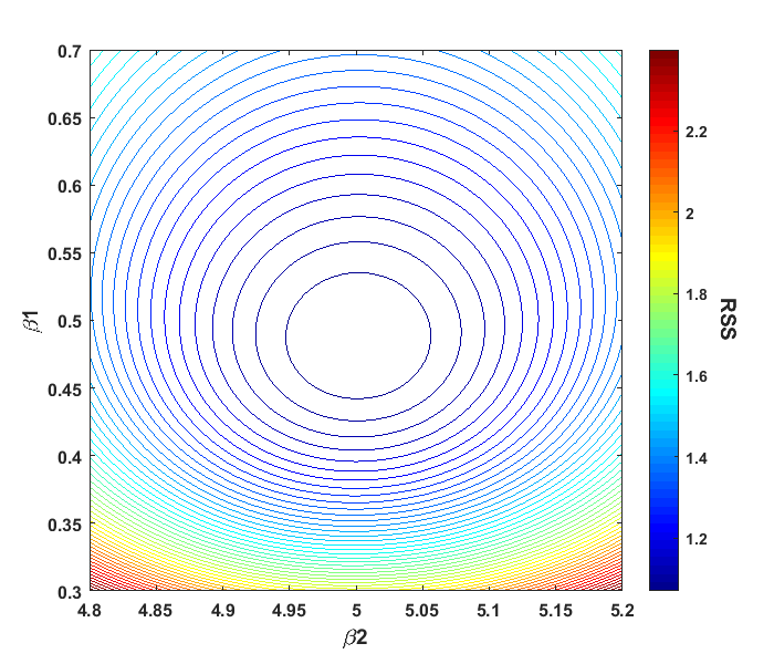
This plot shows that the innermost contour is close to circular when plotting both β parameters on the same scale. These contour patterns are useful for gaining insight into what values future parameter estimates are likely to assume and how these values will be distributed. More on that in a moment. We now return to our covariance matrix as we still have values to examine there. The off-diagonal elements tell us how much β1 and β2 co-vary or vary together. A covariance matrix is symmetric, meaning the off-diagonal elements will be equal. The covariance between our two β parameters (0.0000011) is much lower than either of the individual parameter variances, suggesting that there is little covariance between the two parameters. Typically, the relation between two parameters is often viewed instead as a correlation, with Pearson’s correlation coefficient being the most common measure used. Pearson’s coefficient is a normalized value of correlation on a scale of 0 to 1, with 0 being no correlation and 1 full correlation. Converting the covariance matrix to a correlation matrix is fairly easy
DiagCov = 1 ./ sqrt(diag(CovMatrix));
DiagCorr = spdiags(DiagCov,0,NumParams,NumParams);
CorrMatrix = DiagCorr * CovMatrix * DiagCorr

CorrMatrix =

    1.0000    0.0011
    0.0011    1.0000
The diagonal elements of the correlation matrix are always 1, since a variable has full correlation with itself. We can also see that the correlation coefficient between the two β parameters is effectively zero. This is a good thing and I will explain why. A regression algorithm is solving the inverse problem of determining the parameter values given a set of data. If a particular model has a high correlation between its parameters, then the algorithm will have a more difficult time distinguishing between the two parameters. In a linear model, highly correlated parameters produce a phenomenon known as collinearity (sometimes called multicollinearity). Let’s say that we used a linear model y = 2x + ε to generate a set of noisy data and to fit our model with a regression algorithm we use
y = ax + bx + ε
It’s easy to see here that the factor bx is redundant as there is already a parameter which has a linear relationship between y and x, a. But, if this model is used in a regression algorithm, we are effectively giving it the problem
y = (a + b)x + ε
Or solving the underdetermined equation, a + b = 2, of which there are an infinite number of solutions. This is why examining our models for parameter correlation is so important. If we apply such a model in this situation, the regression matrix will be ill-conditioned, causing large uncertainty in the values of the parameter estimates. More importantly, if only R2 or other goodness-of-fit measures are used to check the results of the regression algorithm, there will be no indication of any parameter estimate problems. If correlation issues with the parameters show up in a nonlinear model, the circular/elliptical contour shapes shown above will be instead irregular and erratic, meaning that the distribution of estimates over repeated measurements may not form a normal distribution.
I discuss these parameter estimation problems in my PhD Thesis, specifically what happens when these problems manifest themselves in nonlinear models and how to better diagnose when they exist. If you are interested in learning more about NLLS regression, including parameter estimation issues, I found these references to be handy.
References and Reading Material
Nonlinear Regression by Seber and Wild
This is the “bible” on nonlinear regression and discusses issues with ill-conditioning and parameter contours. It is math intensive, and it took me several iterations to grasp some topics, but it is very comprehensive. I had this book checked out from the library for months, but it is nice to see an electronic copy is now available if your library or organization has access rights.
Nonlinear Regression Analysis and Its Applications by Bates and Watts
Very similar style to Seber and Wild, but this book is more approachable and uses the same several model/data problem sets throughout the book, which is helpful for learning. Also now available electronically.
Nonlinear Parameter Optimization Using R Tools by John C. Nash
Referenced above, but I found it so useful that I’m repeating it here.